Solady's cbrt, derived: The cost of broken symmetry and the 0x90b5e5 magic constant
Special thanks to Duncan for the original implementation in 0x-settler/Cbrt.sol.
There is a number sitting in the middle of Solady’s cbrt with no comment, no link, and no explanation: 0x90b5e5. It is packed into a one-byte table lookup that runs before any real math happens. Remove it and the function still works — it just runs about 40% slower.
This post is about what that number is, why it exists, and why nothing like it appears in the sqrt function we worked through last time. The short version: square root has a hidden symmetry that makes magic constants pointless. Cube root doesn’t. 0x90b5e5 is the exact price of that broken symmetry.
Understanding this saves you from the trap of thinking optimized math code is just “bit tricks” — there’s a clean theory underneath, and once you see it, you can derive these constants yourself for any root.
TL;DR: Cube root’s Newton method punishes underestimates much harder than overestimates (unlike square root, which treats them equally). The constant
0x90b5e5packs three correction factors — one per remainder class of the input’s bit-length mod 3 — that rebalance each case so no starting guess is too far off. This turns 7 Newton iterations into 5, saving ~160 gas for ~10 gas of setup.
Here is the implementation from Solady’s FixedPointMathLib:
/// Credit to duncancmt
/// https://github.com/0xProject/0x-settler/blob/2577ae61a3ca26a5b37ef8769b05f05de5115e93/src/vendor/Cbrt.sol
function cbrt(uint256 x) internal pure returns (uint256 z) {
    /// @solidity memory-safe-assembly
    assembly {
        let b := sub(255, clz(x))
        z := or(shr(7, shl(div(b, 3), byte(add(mod(b, 3), 29), 0x90b5e5))), 1)
        // 5 Newton-Raphson iterations
        z := div(add(add(div(x, mul(z, z)), z), z), 3)
        z := div(add(add(div(x, mul(z, z)), z), z), 3)
        z := div(add(add(div(x, mul(z, z)), z), z), 3)
        z := div(add(add(div(x, mul(z, z)), z), z), 3)
        z := div(add(add(div(x, mul(z, z)), z), z), 3)
        // Round down
        z := sub(z, lt(div(x, mul(z, z)), z))
    }
}
Same shape as sqrt — initial guess, Newton iterations, floor correction. But two things stand out:
- The initial guess hides a magic constant inside
0x90b5e5. Square root had no such thing. - There are 5 Newton iterations, not 6.
These two facts are the same fact. The constant is what makes 5 iterations enough; without it you’d need 7. Everything that follows shows, step by step, why that number has to exist and why those exact three bytes are the right ones.
The target is floor(∛x) for any x up to \(2^{256} - 1\). Since \(\lfloor\sqrt[3]{2^{256} - 1}\rfloor \approx 2^{85.33}\), the answer fits in at most 86 bits — that’s our precision budget. Sqrt needed 128 bits; cube root needs less, which leaves room to be clever about iterations.
Bounding the cube root
Let \(n = \lfloor\log_2(x)\rfloor\) — the position of the highest set bit. By definition:
\[2^n \le x < 2^{n+1}\]Taking the cube root:
\[2^{n/3} \le \sqrt[3]{x} < 2^{(n+1)/3} \quad \text{--- (eq. 1)}\]The true cube root is squeezed between two powers of 2, and the gap between them is always a factor of \(2^{1/3} \approx 1.26\). That’s enough to nail down a starting guess — but as we’ll see, which power of 2 we pick matters a lot.
The initial guess and three error buckets
A natural starting guess comes from the bound above. Since \(\sqrt[3]{x} \approx 2^{n/3}\), we can try:
\[z_0 = 2^{\lfloor(n+1)/3\rfloor}\]This is the cube root analog of the sqrt post’s initial guess \(2^{\lfloor(n+1)/2\rfloor}\) — take the bit position, add 1, divide by 3, round down, and raise 2 to that power.
Because we divide by 3, the exact behavior depends on the remainder when \(n\) is divided by 3. There are three cases.
For each, we’ll track two quantities. The first is the ratio of our guess to the truth:
\[r_0 = \frac{z_0}{\sqrt[3]{x}}\]The second is the relative error — the standard definition, “how far off as a fraction of the truth”:
\[\varepsilon_0 = \frac{\text{approximation} - \text{true value}}{\text{true value}} = \frac{z_0 - \sqrt[3]{x}}{\sqrt[3]{x}} = \frac{z_0}{\sqrt[3]{x}} - 1 = r_0 - 1\]So \(\varepsilon_0\) is just \(r_0\) shifted down by 1. Once we know the range of \(r_0\), we get the range of \(\varepsilon_0\) by subtracting 1 from both endpoints.
Case 0: \(n \bmod 3 = 0\)
Write \(n = 3k\). Then:
\[z_0 = 2^{\lfloor(3k+1)/3\rfloor} = 2^k\]From equation (1), the true cube root lies in \([2^k, \; 2^k \cdot 2^{1/3})\). The ratio is:
\[r_0 = \frac{z_0}{\sqrt[3]{x}} = \frac{2^k}{[2^k, \; 2^k \cdot 2^{1/3})} \;\in\; (2^{-1/3}, \; 1] \;=\; (0.794, \; 1]\]The ratio is below 1 — an underestimate. Subtracting 1:
\[\varepsilon_0 = r_0 - 1 \;\in\; (0.794 - 1, \; 1 - 1] \;=\; (-0.206, \; 0]\]Worst case: \(\lvert\varepsilon_0\rvert = 0.206\).
Case 1: \(n \bmod 3 = 1\)
Write \(n = 3k + 1\). Then:
\[z_0 = 2^{\lfloor(3k+2)/3\rfloor} = 2^k\]Same \(z_0\) as Case 0! But now the true cube root lies in a higher range: \([2^k \cdot 2^{1/3}, \; 2^k \cdot 2^{2/3})\). So the ratio is smaller:
\[r_0 = \frac{2^k}{[2^k \cdot 2^{1/3}, \; 2^k \cdot 2^{2/3})} \;\in\; (2^{-2/3}, \; 2^{-1/3}] \;=\; (0.630, \; 0.794]\]A deeper underestimate. Subtracting 1:
\[\varepsilon_0 = r_0 - 1 \;\in\; (0.630 - 1, \; 0.794 - 1] \;=\; (-0.370, \; -0.206]\]Worst case: \(\lvert\varepsilon_0\rvert = 0.370\).
Case 2: \(n \bmod 3 = 2\)
Write \(n = 3k + 2\). Then:
\[z_0 = 2^{\lfloor(3k+3)/3\rfloor} = 2^{k+1}\]Now \(z_0\) jumps up by a factor of 2 compared to Cases 0 and 1. The true cube root lies in \([2^k \cdot 2^{2/3}, \; 2^{k+1})\). The ratio:
\[r_0 = \frac{2^{k+1}}{[2^k \cdot 2^{2/3}, \; 2^{k+1})} \;\in\; (1, \; 2^{1/3}] \;=\; (1, \; 1.260]\]An overestimate — the only case where our guess is above the true answer. Subtracting 1:
\[\varepsilon_0 = r_0 - 1 \;\in\; (1 - 1, \; 1.260 - 1] \;=\; (0, \; 0.260]\]Worst case: \(\lvert\varepsilon_0\rvert = 0.260\).
The combined picture
| Case (\(n \bmod 3\)) | \(z_0\) | Ratio range | Error range | Worst \(\lvert\varepsilon_0\rvert\) | Type |
|---|---|---|---|---|---|
| 0 | \(2^k\) | \((0.794, \; 1]\) | \((-0.206, \; 0]\) | 0.206 | underestimate |
| 1 | \(2^k\) | \((0.630, \; 0.794]\) | \((-0.370, \; -0.206]\) | 0.370 | underestimate |
| 2 | \(2^{k+1}\) | \((1, \; 1.260]\) | \((0, \; 0.260]\) | 0.260 | overestimate |
Case 1 is the bottleneck — always an underestimate, worst error 0.370, only 1.43 bits of accuracy. Our three starting points range from “pretty close” to “dangerously far off” — and it’s the worst one that decides how many iterations we need.
But hold on — is being an underestimate actually worse than being an overestimate of the same size? For sqrt the answer was no, they’re identical. For cbrt, as we’re about to see, the answer is very much yes.
The Newton-Raphson iteration
We want \(z\) such that \(z^3 = x\). Define \(f(z) = z^3 - x\), with derivative \(f’(z) = 3z^2\). Newton-Raphson gives:
\[z_{n+1} = z_n - \frac{z_n^3 - x}{3z_n^2}\]Simplifying:
\[z_{n+1} = \frac{2z_n^3 + x}{3z_n^2} = \frac{2z_n}{3} + \frac{x}{3z_n^2}\]So the cube root Newton step is:
\[\boxed{\;z_{n+1} = \frac{2z_n + x/z_n^2}{3}\;}\]In plain English: take twice the current guess, add \(x\) divided by the guess squared, then divide everything by 3.
In Solady’s code, div(add(add(div(x, mul(z, z)), z), z), 3) does exactly this: mul(z, z) is \(z^2\), div(x, ...) is \(x/z^2\), adding z twice gives \(2z + x/z^2\), and div(..., 3) finishes it.
Compare with sqrt’s formula \((z + x/z)/2\). Two differences: we multiply \(z\) by 2 instead of 1, and we divide by \(z^2\) instead of \(z\). Both matter in the error analysis.
The exact error formula (and the broken symmetry)
Substituting \(z_n = (1 + \varepsilon_n) \cdot \sqrt[3]{x}\) into the Newton step and working through the algebra, we get the exact error recurrence:
\[\boxed{\;\varepsilon_{n+1} = \frac{\varepsilon_n^2 \; (3 + 2\varepsilon_n)}{3 \; (1 + \varepsilon_n)^2}\;}\]Compare with sqrt’s formula: \(\varepsilon_{n+1} = \varepsilon_n^2 / (2(1 + \varepsilon_n))\).
Both are quadratic — the error gets squared each step, so bits of accuracy roughly double. That’s the good news.
The bad news: cube root’s formula is not symmetric. In the sqrt post, the Newton map satisfied \(g(r) = g(1/r)\) — an overestimate by a factor of 2 corrected exactly the same as an underestimate by a factor of 2.
Does that hold for cube root? The ratio map is \(g(r) = (2r + 1/r^2)/3\). Let’s check:
\[g(2) = \frac{4 + 0.25}{3} \approx 1.417\] \[g(1/2) = \frac{1 + 4}{3} \approx 1.667\]Not equal. The symmetry is gone. Halving your guess costs you more than doubling it. The \(1/r^2\) term — from the \(x/z^2\) in Newton’s step — punishes small \(r\) much harder than it punishes large \(r\). This single broken equality is the entire reason 0x90b5e5 exists.
The graph below shows this visually. The blue curve (sqrt) is nearly symmetric around \(\varepsilon = 0\), while the orange curve (cbrt) tilts sharply upward for negative errors:
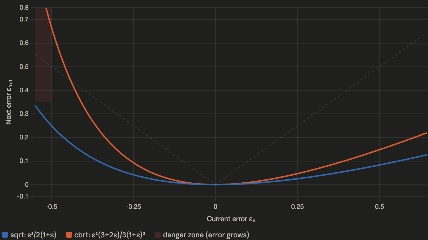 The cbrt error curve (orange) rises sharply for negative \(\varepsilon\) (underestimates), while the sqrt curve (blue) stays symmetric. The dashed line marks \(\lvert\varepsilon_{n+1}\rvert = \lvert\varepsilon_n\rvert\) — above it, errors grow rather than shrink.
Why underestimates are dangerous
Let’s make this concrete with a number. Suppose our guess is half the true answer — \(\varepsilon_0 = -0.5\). Plug in:
\[\varepsilon_1 = \frac{(-0.5)^2 \cdot (3 - 1)}{3 \cdot (0.5)^2} = \frac{0.25 \times 2}{0.75} \approx 0.667\]0.5 in, 0.667 out. You asked Newton to fix your guess, and it handed you back something worse. The \(1/r^2\) term blows up when \(r\) is small — at \(r = 0.5\), it gives 4, which Newton then plugs straight into the next guess. It’s like asking for directions and being sent further from your destination.
Sqrt’s symmetry made sure the correction was equal in both directions, so this couldn’t happen. Cube root has no such safety net, and any algorithm that doesn’t account for it will waste iterations.
The asymmetry tax: a wasted first step
Now look back at our three cases. Case 1 starts with \(\varepsilon_0 = -0.370\) (an underestimate). After one Newton step:
\[\varepsilon_1 = \frac{(-0.370)^2 \cdot (3 + 2(-0.370))}{3 \cdot (1 - 0.370)^2} = \frac{0.137 \times 2.26}{3 \times 0.397} \approx +0.260\]The error went from \(-0.370\) to \(+0.260\). In terms of \(\lvert\varepsilon\rvert\): from 0.370 down to 0.260. Only a small improvement — from 1.43 bits to 1.94 bits.
Compare: Case 2 starts at \(\varepsilon_0 = +0.260\) (an overestimate of the same size). After one Newton step:
\[\varepsilon_1 = \frac{(0.260)^2 \cdot (3 + 0.520)}{3 \cdot (1.260)^2} \approx 0.050\]From \(0.260\) down to \(0.050\). That’s 1.94 bits jumping to 4.32 bits — a huge improvement.
Case 1 spends its entire first Newton step just getting back to where Case 2 already started. After step 1, Case 1’s error is \(+0.260\) — exactly Case 2’s starting point. From there both cases follow the same path. It’s like running a race where one runner has to jog back to the starting line before they can actually begin.
That’s the asymmetry tax: a full Newton iteration, paid only by underestimates, while overestimates get the same progress for free.
How many iterations to reach 86 bits?
The worst case is Case 1 (\(\varepsilon_0 = -0.370\)). Let’s trace Newton’s convergence:
| Step | Error (\(\varepsilon\)) | Bits of accuracy | Notes |
|---|---|---|---|
| 0 | \(-0.370\) | 1.43 | initial guess (underestimate) |
| 1 | \(+0.260\) | 1.94 | recovered to overestimate (barely improved!) |
| 2 | \(+0.050\) | 4.32 | now converging normally |
| 3 | \(+2.34 \times 10^{-3}\) | 8.74 | |
| 4 | \(+5.45 \times 10^{-6}\) | 17.49 | |
| 5 | \(+2.97 \times 10^{-11}\) | 34.97 | |
| 6 | \(+8.79 \times 10^{-22}\) | 69.95 | ← not enough for 86 |
| 7 | \(+7.73 \times 10^{-43}\) | 139.89 ✓ |
Step 6 gives only 70 bits — short of our 86-bit target. We need step 7 for 140 bits.
With the plain bit-length guess and no other tricks, we need 7 Newton iterations.
(For comparison: Case 2 starting from \(+0.260\) reaches 140 bits at step 6 — only 6 iterations. Case 1’s extra iteration is entirely the asymmetry tax on its underestimate.)
Can we do better?
The naive guess needs 7 iterations. Solady ships with 5. Where do the missing two go?
Look at the three error buckets again:
| Case | Error range | Position relative to \(r = 1\) |
|---|---|---|
| 0 | \((-0.206, \; 0]\) | slightly below 1 |
| 1 | \((-0.370, \; -0.206]\) | well below 1 (danger zone) |
| 2 | \((0, \; 0.260]\) | above 1 (safe zone) |
Three buckets, three completely different starting positions. Case 1 sits deep in the danger zone; Case 0 sits near it; Case 2 lands safely above. The result is very uneven worst-case behavior.
Here’s the trick: multiply each bucket by its own carefully chosen constant to pull its range onto \(r = 1\).
In sqrt, the symmetry made this pointless — any \(c \neq 1\) hurt one side as much as it helped the other. Cube root has no such constraint. Each remainder is independent, so each gets its own best multiplier. Three buckets, three constants, packed into three bytes.
Deriving the three magic constants
Step 1: Give each bucket its own boost
Think of it like this. You have three groups of inputs, and for each group, your guess lands in a different spot relative to the true answer:
- Bucket 0: Your guess is 79–100% of the truth (not bad)
- Bucket 1: Your guess is 63–79% of the truth (too low — danger zone)
- Bucket 2: Your guess is 50–63% of the truth (way too low)
What if, before running Newton’s method, you multiplied your guess by a small correction factor? A different factor for each bucket, chosen so that every bucket lands in the same sweet spot?
Picture a number line with 1.0 in the middle (a perfect guess). Each bucket is a range sitting to the left of 1.0. We want to slide each range so it’s centered on 1.0 — half overestimating, half underestimating, by equal amounts.
To make this work cleanly in the code (and avoid branches in the assembly), we first force the base guess to use the same formula for all three cases: just \(2^{\lfloor n/3 \rfloor}\) (which is \(2^k\)). Then we put ALL the adjustment burden onto a per-bucket multiplier:
\[z_0 = c_s \cdot 2^{\lfloor n/3 \rfloor}\]Here \(c_s\) is a multiplier that depends on \(s = n \bmod 3\).
Why \(\lfloor n/3 \rfloor\) instead of the naive \(\lfloor(n+1)/3\rfloor\)? Gas. In EVM assembly, computing
div(n, 3)costs less than computingdiv(add(n, 1), 3). Since we are going to use a table lookup for the multiplier \(c_s\) anyway, we can just bake the mathematical difference directly into the multiplier constants and save an instruction!
To see exactly where the base bounds come from, remember that if \(n = 3k + s\), then \(x\) spans from \(2^{3k+s}\) up to \(2^{3k+s+1}\). This means the true cube root \(\sqrt[3]{x}\) spans from \(2^{k+s/3}\) up to \(2^{k+(s+1)/3}\).
Since our base guess is fixed at \(2^k\), dividing the guess by those true bounds gives us the general baseline ratio range: \((2^{-(s+1)/3}, \; 2^{-s/3}]\).
Plugging in \(s \in {0, 1, 2}\) gives us the exact baseline ratios before any multipliers are applied:
| \(s\) | Base ratio \(r_0 \in (2^{-(s+1)/3}, \; 2^{-s/3}]\) |
|---|---|
| 0 | \((2^{-1/3}, \; 2^0]\) = \((0.794, \; 1.000]\) |
| 1 | \((2^{-2/3}, \; 2^{-1/3}]\) = \((0.630, \; 0.794]\) |
| 2 | \((2^{-1}, \; 2^{-2/3}]\) = \((0.500, \; 0.630]\) |
Without multipliers, all three buckets are underestimates (\(r_0 \le 1\)). That’s the danger zone. The multiplier \(c_s\) will lift each one so its error is properly centered.
Step 2: The centering condition
After multiplying by \(c_s\), the range \((a, b]\) becomes \((c_s \cdot a, \; c_s \cdot b]\). We want this centered on \(r = 1\) — meaning the error at the low end and the error at the high end are equal in size (one negative, one positive).
What does “centered” mean here? Since we’re dealing with ratios, the right notion of “center” is the geometric mean, not the arithmetic mean. If your range runs from a to b, you want the multiplier c such that c·a is as far below 1 as c·b is above 1 — on a log scale. It’s the same idea as rebalancing a seesaw: find the midpoint (geometrically), and shift everything so that midpoint sits on 1.
The new endpoints \(c_s \cdot a\) and \(c_s \cdot b\) are centered on 1 when their logs add to zero:
\[\log_2(c_s \cdot a) + \log_2(c_s \cdot b) = 0\]This means \(c_s^2 \cdot a \cdot b = 1\), so:
\[\boxed{\;c_s = \frac{1}{\sqrt{a \cdot b}}\;}\]The optimal multiplier is 1 divided by the geometric mean of the range endpoints.
Step 3: Plug in each bucket
\(s = 0\), range \((a, b] = (2^{-1/3}, \; 1]\):
\[c_0 = \frac{1}{\sqrt{2^{-1/3} \cdot 1}} = \frac{1}{2^{-1/6}} = 2^{1/6} \approx 1.1225\]\(s = 1\), range \((a, b] = (2^{-2/3}, \; 2^{-1/3}]\):
\[c_1 = \frac{1}{\sqrt{2^{-2/3} \cdot 2^{-1/3}}} = \frac{1}{\sqrt{2^{-1}}} = 2^{1/2} = \sqrt{2} \approx 1.4142\]\(s = 2\), range \((a, b] = (2^{-1}, \; 2^{-2/3}]\):
\[c_2 = \frac{1}{\sqrt{2^{-1} \cdot 2^{-2/3}}} = \frac{1}{\sqrt{2^{-5/3}}} = 2^{5/6} \approx 1.7818\]Three beautiful numbers: \(2^{1/6}\), \(2^{3/6}\), \(2^{5/6}\) — evenly spaced on a log scale (each one is a factor of \(2^{1/3}\) bigger than the previous).
Step 4: Verify the centered ranges
Applying our multipliers shifts all three buckets into the exact same balanced range:
\[\begin{aligned} s = 0: \quad & (2^{-1/3} \cdot 2^{1/6}, \;\; 1 \cdot 2^{1/6}] &= (2^{-1/6}, \; 2^{1/6}] \\ s = 1: \quad & (2^{-2/3} \cdot 2^{1/2}, \;\; 2^{-1/3} \cdot 2^{1/2}] &= (2^{-1/6}, \; 2^{1/6}] \\ s = 2: \quad & (2^{-1} \cdot 2^{5/6}, \;\; 2^{-2/3} \cdot 2^{5/6}] &= (2^{-1/6}, \; 2^{1/6}] \end{aligned}\]Because they all map to \((2^{-1/6}, \; 2^{1/6}]\), the initial ratio \(r_0\) is bounded exactly the same way regardless of the remainder:
\[r_0 \in (0.891, \; 1.122] \implies \lvert\varepsilon_0\rvert \le 0.122\]The per-remainder multipliers have made the error the same in every case.
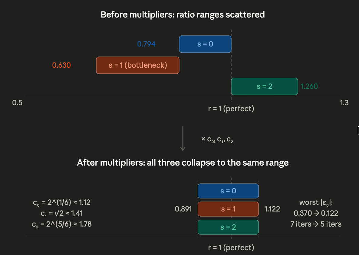 Before multipliers (top): three buckets scattered across different positions relative to \(r = 1\). After multipliers (bottom): all three collapse to the same narrow range centered on \(r = 1\). Worst error drops from 0.370 to 0.122.
| Before multipliers | After multipliers | |
|---|---|---|
| Worst \(\lvert\varepsilon_0\rvert\) | 0.370 (1.43 bits) | 0.122 (3.03 bits) |
| Underestimate risk | Case 1 deep in danger zone | All buckets balanced |
A 1.6-bit improvement from a one-byte lookup.
From real numbers to 0x90b5e5
These ideal multipliers are irrational numbers (numbers like \(\sqrt{2}\) that can’t be written as a fraction). But the EVM only does integer math. So how do we actually use them?
The trick is fixed-point arithmetic: multiply each constant by 128 (a power of 2), round to the nearest integer, and later divide by 128 using a cheap bit shift.
Let’s walk through one example completely. Take bucket 0: the ideal multiplier is \(2^{1/6} \approx 1.1225\). Multiply by 128: \(1.1225 \times 128 = 143.68\), which rounds to 144, or 0x90 in hex. That’s our first byte.
Do the same for the other two buckets:
| \(s\) | Optimal \(c_s\) | \(c_s \times 128\) | Rounded | Hex |
|---|---|---|---|---|
| 0 | \(2^{1/6} \approx 1.1225\) | 143.68 | 144 | 0x90 |
| 1 | \(\sqrt{2} \approx 1.4142\) | 181.02 | 181 | 0xb5 |
| 2 | \(2^{5/6} \approx 1.7818\) | 228.07 | 229 | 0xe5 |
Concatenate the three bytes and you get 0x90b5e5. That’s the magic constant — three carefully derived correction factors, packed into 3 bytes.
How the code uses it
let b := sub(255, clz(x))
z := or(shr(7, shl(div(b, 3), byte(add(mod(b, 3), 29), 0x90b5e5))), 1)
Step by step:
mod(b, 3)— finds the remainder \(s\) (which bucket?).byte(add(s, 29), 0x90b5e5)— picks the right byte. In the EVM,byte()reads from a 32-byte word. The constant0x90b5e5sits in the last 3 bytes: byte 29 is0x90(144), byte 30 is0xb5(181), byte 31 is0xe5(229).shl(div(b, 3), ...)— multiplies the byte by \(2^{\lfloor n/3 \rfloor}\).shr(7, ...)— divides by 128 (the denominator of our fixed-point fraction).or(..., 1)— ensures \(z \ge 1\) when the shift would produce 0.
The result is:
\[z_0 = \frac{c_s}{128} \cdot 2^{\lfloor n/3 \rfloor}\]In one line: figure out which bucket you’re in, grab the right byte from the constant, multiply it by the power-of-two base, and divide by 128 to undo the fixed-point scaling. Seven opcodes, three multipliers, no branches.
Why exactly 5 iterations now?
With the multipliers, our worst-case starting error drops from 0.370 to ~0.123. Let’s trace:
| Step | Error (\(\varepsilon\)) | Bits of accuracy |
|---|---|---|
| 0 | 0.123 | 3.03 |
| 1 | 0.0129 | 6.28 |
| 2 | \(1.63 \times 10^{-4}\) | 12.58 |
| 3 | \(2.66 \times 10^{-8}\) | 25.16 |
| 4 | \(7.08 \times 10^{-16}\) | 50.33 |
| 5 | \(5.02 \times 10^{-31}\) | 100.65 ✓ |
We need ~86 bits. Step 5 gives 100 bits. Done.
- 4 iterations → 50 bits. Not enough.
- 6 iterations → 200+ bits. Wasted gas.
- 5 iterations is the smallest number that works.
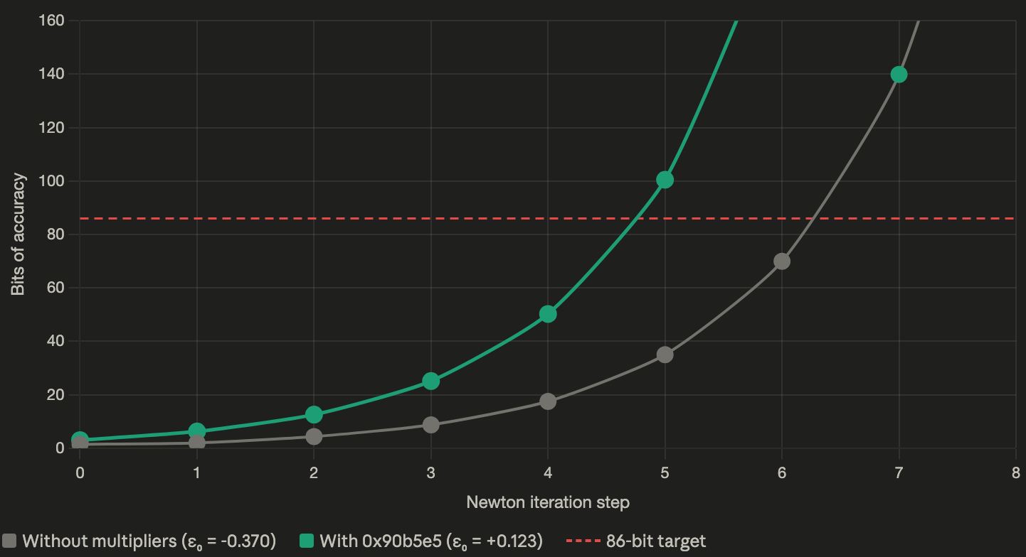 Gray line: without multipliers, starting from \(\varepsilon_0 = -0.370\), the convergence is slow at first (wasted step recovering from underestimate) and crosses 86 bits only at step 7. Green line: with
 0x90b5e5 multipliers, starting from \(\varepsilon_0 = 0.123\), convergence is fast and crosses 86 bits at step 5.
The full comparison
| Without multipliers | With 0x90b5e5 |
|
|---|---|---|
| Worst \(\lvert\varepsilon_0\rvert\) | 0.370 (1.43 bits) | 0.123 (3.03 bits) |
| Worst case | Case 1 underestimate | All cases balanced |
| Iterations needed | 7 | 5 |
The three magic constants saved 2 full Newton iterations — roughly 160 gas — for the cost of a single byte-lookup (~10 gas of setup).
And notice where those 2 iterations come from. Without multipliers, Case 1 wastes one step recovering from its underestimate, and then needs 6 more to finish — 7 total. The multipliers got rid of that wasted step by centering Case 1’s range on \(r = 1\), AND made the starting accuracy good enough that 5 steps are enough instead of 6.
The floor correction
z := sub(z, lt(div(x, mul(z, z)), z))
This works the same way as in the sqrt post:
mul(z, z)computes \(z^2\).div(x, z²)computes \(x / z^2\).lt(x/z², z)checks: is \(x/z^2 < z\)? That’s the same as \(x < z^3\) — did we overshoot?- If yes, subtract 1 from \(z\).
Just like sqrt, integer cube root can end up one above the true floor. This single line catches it.
Why sqrt can’t use this trick (and cbrt can)
For square root, the Newton map satisfies \(g(r) = g(1/r)\). This forced the optimal magic constant to be 1 — any \(c \neq 1\) makes one side worse by exactly the amount it makes the other side better.
For cube root, the Newton map is \(g(r) = (2r + 1/r^2)/3\). We showed \(g(2) \approx 1.417\) while \(g(1/2) \approx 1.667\). The symmetry is gone. Overestimates and underestimates are treated differently.
This broken symmetry is what opens the door for the multipliers. With no symmetry forcing \(c = 1\), we’re free to pick different constants per bucket. The broken symmetry is the reason 0x90b5e5 exists.
Generalizing: Newton-Raphson for any \(k\)-th root
The pattern from these two posts isn’t specific to square and cube roots. It generalizes cleanly to any \(k\)-th root.
The general Newton formula
To find \(x^{1/k}\), we want the root of \(f(z) = z^k - x\). The derivative is \(f’(z) = kz^{k-1}\). Newton-Raphson gives:
\[z_{n+1} = z_n - \frac{z_n^k - x}{kz_n^{k-1}} = \frac{(k-1)z_n^k + x}{kz_n^{k-1}} = \frac{(k-1)z_n + x/z_n^{k-1}}{k}\]So the general formula is:
\[\boxed{\;z_{n+1} = \frac{(k-1) \cdot z + x/z^{k-1}}{k}\;}\]Check: for \(k = 2\), this gives \((z + x/z)/2\) (sqrt). For \(k = 3\), it gives \((2z + x/z^2)/3\) (cbrt). ✓
The general ratio recurrence
Substituting \(z = r \cdot x^{1/k}\) and simplifying (the \(x\) cancels as always):
\[r_{n+1} = \frac{(k-1) \cdot r + 1/r^{k-1}}{k}\]The symmetry test
Define \(g_k(r) = ((k-1)r + 1/r^{k-1})/k\). Is \(g_k(r) = g_k(1/r)\)?
\[g_k(1/r) = \frac{(k-1)/r + r^{k-1}}{k}\]For this to equal \(g_k(r) = ((k-1)r + 1/r^{k-1})/k\), we need:
\[(k-1)/r + r^{k-1} = (k-1)r + 1/r^{k-1}\]Rearranging: \((k-1)(1/r - r) = 1/r^{k-1} - r^{k-1}\). The left side is \((k-1)(1/r - r)\). The right side is \((1/r^{k-1} - r^{k-1})\).
For \(k = 2\): LHS = \((1/r - r)\), RHS = \((1/r - r)\). Equal. ✓ Symmetry holds.
For \(k = 3\): LHS = \(2(1/r - r)\), RHS = \((1/r^2 - r^2) = (1/r - r)(1/r + r)\). These are equal only if \(1/r + r = 2\), i.e., \(r = 1\). Not equal in general. ✗
For \(k \ge 3\): the right side grows as \(r^{k-1}\), the left side grows as \(r\). They can’t match. Symmetry always breaks.
The general recipe
This gives us a complete recipe for implementing any \(k\)-th root:
| Property | \(k = 2\) (sqrt) | \(k \ge 3\) |
|---|---|---|
| Symmetry \(g(r) = g(1/r)\) | ✓ holds | ✗ broken |
| Magic constants useful? | No (optimal \(c = 1\)) | Yes |
| Number of multipliers | 0 | \(k\) (one per \(n \bmod k\)) |
| Multiplier for bucket \(s\) | — | \(c_s = 2^{(2s+1)/2k}\) |
| Bits of accuracy per bucket | \(\approx 1.27\) (bit-length only) | \(\approx -\log_2(2^{1/2k} - 1)\) |
The general multiplier formula \(c_s = 2^{(2s+1)/2k}\) comes from the same geometric-centering derivation we did for cbrt, applied to the \(k\)-bucket case where each bucket has width \(1/k\) on the log scale.
Let’s verify for cbrt (\(k = 3\)):
- \(s = 0\): \(c_0 = 2^{1/6}\) ✓
- \(s = 1\): \(c_1 = 2^{3/6} = 2^{1/2} = \sqrt{2}\) ✓
- \(s = 2\): \(c_2 = 2^{5/6}\) ✓
And the per-bucket error after centering is always \(2^{1/2k} - 1\):
- \(k = 3\): \(2^{1/6} - 1 \approx 0.122\) ✓
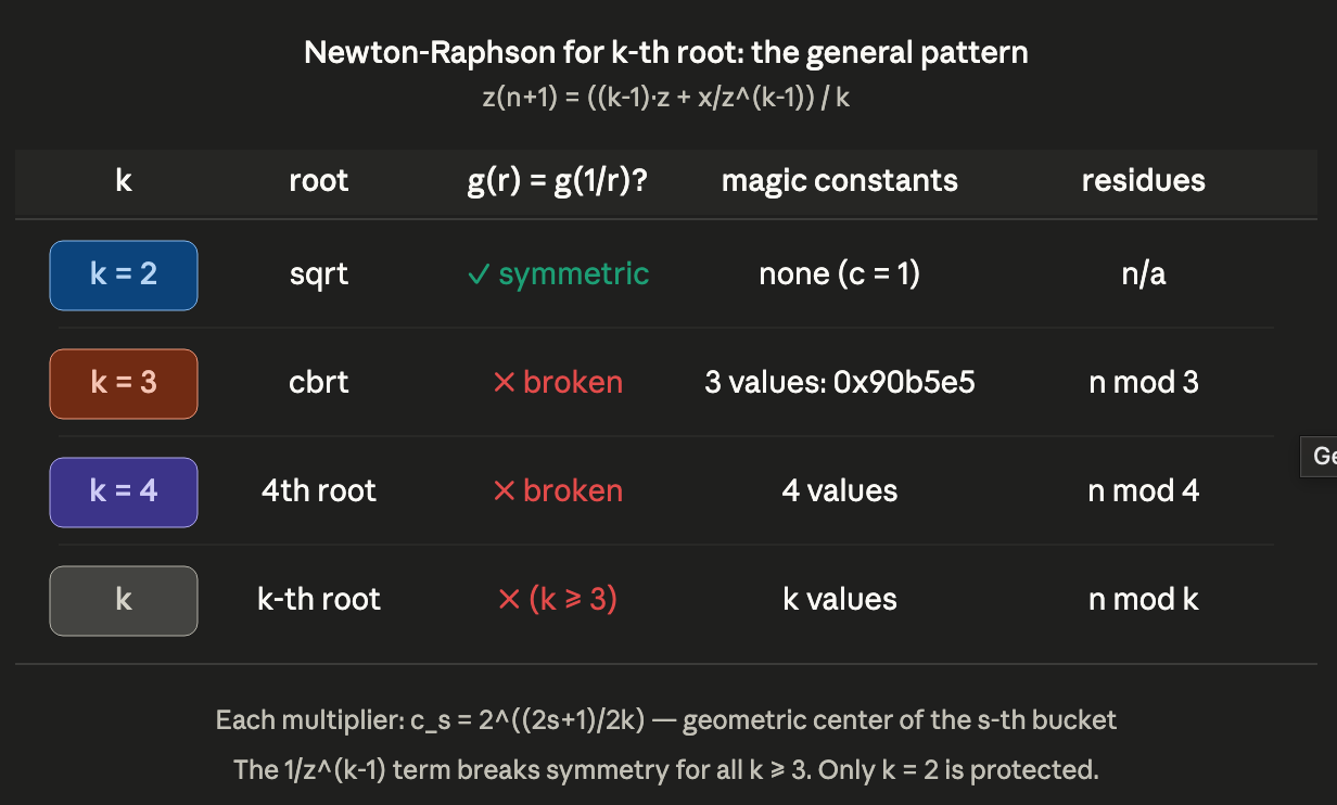 The Newton-Raphson pattern for k-th roots. Only \(k = 2\) (sqrt) has the symmetry that makes magic constants useless. All \(k \ge 3\) benefit from \(k\) per-residue multipliers, each derived from the geometric center of its bucket.
The error formula generalizes too
For the \(k\)-th root, the exact error recurrence (derivable by the same substitution method) has the form:
\[\varepsilon_{n+1} = \frac{\varepsilon_n^2 \cdot P_k(\varepsilon_n)}{k \cdot (1 + \varepsilon_n)^{k-1}}\]where \(P_k\) is a polynomial of degree \(k - 2\). For small \(\varepsilon\):
\[\varepsilon_{n+1} \approx \frac{k-1}{2k} \cdot \varepsilon_n^2\]The constant \((k-1)/2k\) controls the convergence speed:
- \(k = 2\): \((1)/4 = 0.25\) → bits formula: \(\text{bits}_{n+1} \approx 2 \cdot \text{bits}_n + 2\)
- \(k = 3\): \((2)/6 = 0.333\) → bits formula: \(\text{bits}_{n+1} \approx 2 \cdot \text{bits}_n + 1.58\)
- \(k = 4\): \((3)/8 = 0.375\) → bits formula: \(\text{bits}_{n+1} \approx 2 \cdot \text{bits}_n + 1.42\)
Higher \(k\) means the constant gets closer to \(1/2\), so convergence is slightly slower per step. But higher \(k\) also means the result has fewer bits (since \(x^{1/k}\) is smaller), so fewer bits are needed. These two effects roughly cancel.
Closing
Solady’s 0x90b5e5 looks like a random number until you see what it actually is: three points evenly spaced on a log scale, each one pulling a different remainder bucket onto the same fixed point. Once you see that, it stops looking magical.
The same recipe works for every \(k\)-th root with \(k \ge 3\): the Newton map’s symmetry breaks, you get \(k\) remainder buckets, and \(c_s = 2^{(2s+1)/2k}\) centers each one. Only square root is special — and it’s special because of a symmetry, not in spite of one.